
SHM for a Mass-Spring E-practical
A realistic 3D virtual physics experiment
Investigation into Simple Harmonic Motion (SHM) using a mass-spring system. The investigation will allow us to determine the spring constant. Change the weight on the spring and time the oscillations - just as with an actual experiment.
Realistic experimental technique
E-practicals are 3d, highly realistic emulations based on a blend of theory and the actual practicals, giving an authentic experience of doing the actual practical in a laboratory. Students operate the apparatus, make measurements and obtain their own results. It is designed to reproduce the experience of performing the practical rather than simply demonstrating the underlying physics. Like a real experiment, it can be done badly. Careless setup or measurements can produce poor results, so students have to apply experimental technique and take care with their measurements.
Useful when laboratory access is limited
Ideal for preparation before a practical, revision afterwards, missed practicals, home study, or demonstrating an experiment when setting up the real apparatus isn't practical.
Works directly in a browser
No installation is required. Windows, Mac and suitable mobile devices can run the WebGL e-practical.
Watch it in Action
Watch a video of the experiment here.
This shows how to use it and how to collect the data.
School/Department licence £9.99
Valid for one year.
Introduction
A coil spring that is firmly attached at the upper end and with a weight attached to the lower end will oscillate up and down with Simple Harmonic Motion (SHM) when given a small downward impulse.
The motion is called harmonic because of its association with the kinds of waves made by musical instruments. For example, the string of a guitar when plucked will move with SHM and this motion is then transferred to the air as sound waves. Perhaps surprisingly any wave can be represented by superimposing a number of different SHM waves. This was discovered by Jean-Baptiste-Joseph Fourier while investigating the heat equation (how heat spreads) and led to the mathematical process of Fourier analysis which can be used to discover all the harmonic components of a wave.
The objective
To investigate how the time-period of a mass-spring system varies under different tensions.
The variables
The weight on the spring is the independent variable. The period of the oscillations is the dependent variable.
The apparatus
-
A weight cradle and set of weights;
-
A coil/helical spring;
-
Length of string;
-
Retort stand and two clamps;
-
G-clamp;
-
A metre rule;
-
A timer.
The Physics
Consider when the spring is stretched from its natural length by a weight and not in motion so that it is in equilibrium, as shown here:

There is the force from the weight acting downwards and the force from the tension in the spring acting upwards. These are equal and opposite, and we can use Hooke’s law to find the tension, so that:
T1 = ke = mg (eq1)
Where k is the spring constant (the constant of proportionality in Hooke’s law) and e is the extension. So an expression for k is:
k = mg/e
When the spring and weight are in motion, we have the situation shown here:

The spring is stretched by an extra amount x and the force upwards is now T2 given by:
T2 = k(e + x)
So ,the net force is given by:
mg – T2 = mg – k(e + x)
Using Newton’s second law, this can be equated to the mass times the acceleration giving:
ma = mg – k(e + x)
From eq1, ke = mg, so we can simplify this equation to:
ma = -kx
This is the hallmark by which we know SHM; there is a restoring force proportional to the movement or displacement. We can rewrite the equation as:
a = -(k/m)x
Which can be compared to the normal equation for SHM, which is:
a = – ω²x
Where:
ω = √(k/m)
The period for SHM is given by:
T = 2П/ ω
Which in this case will be (we just need to put our equation for ω into this formula):
T = 2П√(m/k)
Thus, the theory of SHM tells us that the period is related to the mass and the spring constant by the formula:
T² = 4Π2m/k
Where k is the spring constant, m is the mass, and T is the period for an entire cycle (down from the midpoint, up through the midpoint, and down to the midpoint). This formula can be rearranged to find the spring constant:
k= 4Π2m/T²
If we take measurements of the period of the oscillation for a range of masses and then plot T2 against m, then k will be 4Π2 divided by the gradient.
What the Students do
Move the lower clamp by placing the mouse pointer over the clamp and using the mouse wheel to move the clamp up and down (or drag if using onscreen controls).
Switch the timer on by mouse clicking the leftmost switch on the timer.
Apply a downward impulse by left-clicking on the weight carrier.
You can start timing by clicking on the left button.
Zooming in using the plus/minus or Z/X keys (or using the magnify icon when using onscreen controls) will make it easier to see the motion.
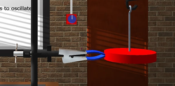
The carrier without extra weights weighs 50 g. Each additional weight is 50 g. You can add weights by moving the mouse over the carrier and using the mouse wheel.
The Results
Note the periods for all possible weights and complete the following table:

When you have completed the table, plot a graph of T² on the Y-axis against m, the mass. This should give you a straight line, which establishes the relationship that the period squared is proportional to the tension in the spring.
Draw the best-fit line through your data points and calculate the gradient.
Use the formula given in the Physics section to calculate the spring constant.
Further Discussion
One could quite easily find the spring constant by measuring the extensions of the spring under some loads. Do this, then compare the value you obtain to one you calculated using the SHM equation for the period.
Which do you think is more accurate, and why?
This section is adapted from material developed by Dr Robert Lucas and is related to the book High School and Undergraduate Physics Practicals, published by CRC Press.